In this post, I walk you through my capstone project for the Metis Data Science Bootcamp, which I completed in the Spring of 2017. The goal of the project was to perform semantic segmentation on satellite images in order to map out farmland around the city of Shanghai.

Why Shanghai?

Here is a side-by-side comparison of Shanghai in 1984 vs. 2016.

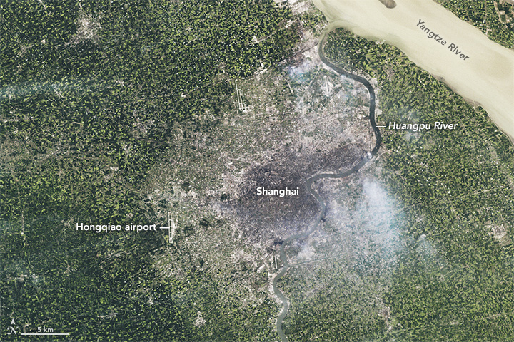
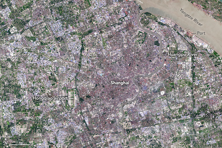
Notice all that green surrounding the little bit of gray in the center of the 1984 image? Yep, that’s mostly forest and farmland. Notice also that it’s almost completely gone in 2016?

That’s why Shanghai.

We’re not setting out on a mission to restore Shanghai to its agricultural glory days. In fact, the modernization of the city is rather impressive. Rather, with this project I wanted to highlight a method that can be used to track farmland, urban development, and natural resources around the world in order to make better decisions for the future of our planet.

The segmentation problem

In addition to the environmental storyline behind this project, I also approached it with the goal to better understand the image segmentation problem. This challenge involves classifying each individual pixel in an image. To do this, current state-of-the-art techniques use a convolutional neural network to first learn the context of progressively coarser regions in an image, and then combine information from different spatial resolutions while upsampling the feature maps back to the size of the original image.

Say what?

Let’s break this process down into two main steps. The first segment of the network uses an image classification backbone, often borrowing from the top classifiers in the ImageNet competition. The classifiers typically contain a series of convolutional layers followed by a pooling layer to reduce the dimensionality. This process is repeated for several stages until you have a dimensionality of, say, 8x8x[num_kernels], with each “pixel” containing semantic information for that region. In classification, this final representation is then reduced to the dimensionality of 8x8x[num_classes] with each 8x8 matrix serving as the feature vector for classifying the entire image, giving you a single probability for each class.

But in segmentation, we don’t simply want a single probability for each class; we want the probability of each class for each pixel in the input image. So if your input image is 224x224, we need classification scores for all 50,176 pixels.

You might see the problem of reducing the image to a 8x8x[whatever] tensor. Let’s say you had a ground truth mask that looked like this:

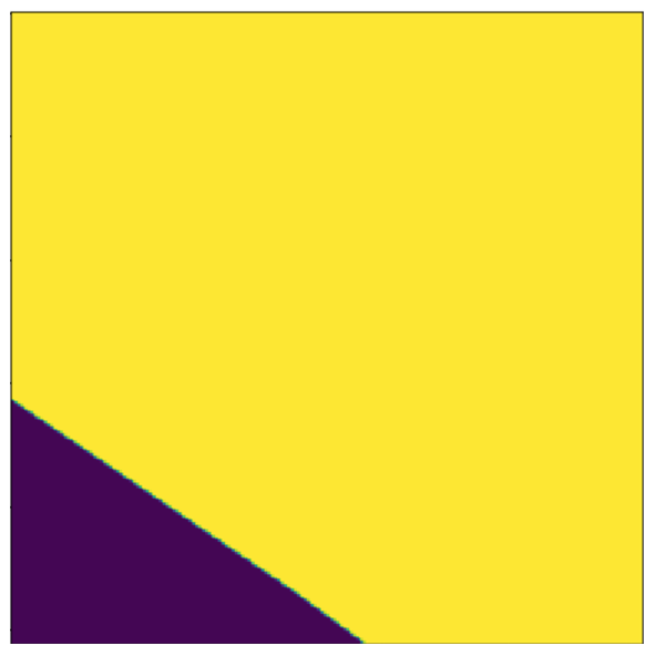
And for the farmland class, you apply a softmax function on the resulting 8x8 feature map to generate class scores that can be interpreted as probabilities of a given region containing farmland. You might get something like this:

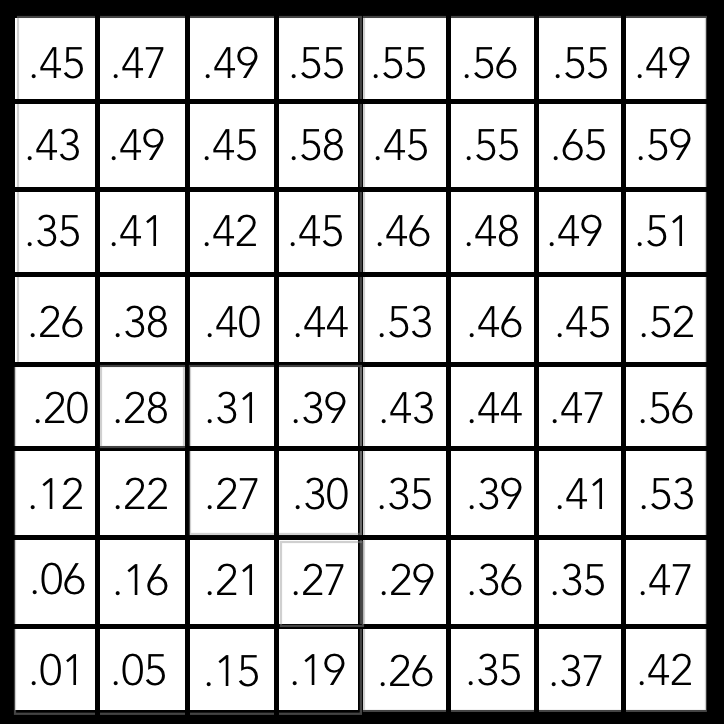
Then with a threshold for positive classification of .25, this would be your resulting prediction:

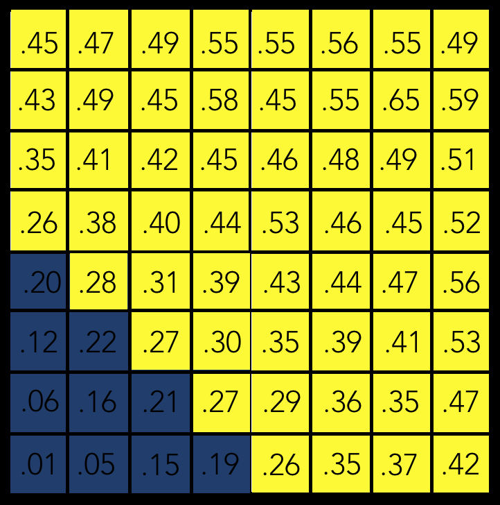
Well, that’s not very precise!

Somehow, we need to make predictions at finer resolutions. One idea would be to altogether avoid any downsampling steps and keep all convolutional layers at the resolution of the input image. The problem with this it will quickly become extremely computationally expensive. For example, running a 3x3 convolution with just 64 filters and a stride of 1 and “same” padding on a 224x224x64 layer would require over 400 million floating point operations for each image in a batch. Not ideal.

Another approach might be to take your 8x8 feature map and do something like bilinear upsampling to go straight back to the original size. But that would throw away far too much information, and we data scientists hate to throw away information when we don’t have to.

The most common solution used in practice is to progressively upsample the feature map that comes out of the classification backbone while adding in information from intermediate feature maps at the different spatial resolutions. I’ll show an example of this in a bit. This process might result in a prediction that looks like this:

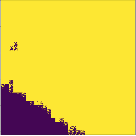
Okay, maybe it’s not the prettiest picture you’ve ever seen, but these are real results that come from combining information from multiple spatial resolutions. This is a trend in image detection and segmentation that has produced remarkable results in practice.

For my project, I played around with two similar approaches to this process. U-NET and FCN.

Perhaps an even more interesting approach that I haven’t yet had the chance to experiment with is Mask R-CNN.

The data

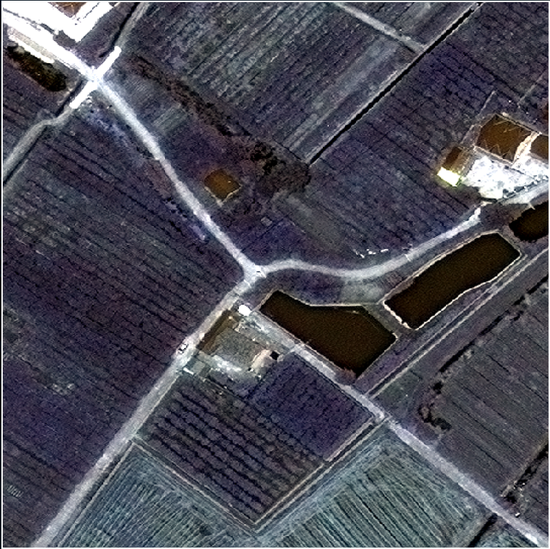
For this project, I utilized images from the SpaceNet dataset taken by Digital Globe’s WorldView-3 satellite. These images were taken at 30cm resolution, which means that one pixel corresponds to 30cm² of actual area. This is the highest resolution earth observation satellite imagery. The project was part of a special partnership with Digital Globe and Metis, in which Alan Schoen (Digital Globe employee and Metis alum) provided an introduction to working with the dataset as well as a primer on dealing with the super fun idiosyncracies of geospatial data.

Exploratory Geospatial Analysis and Creating Ground Truth Masks

At this point, if you are interested in learning more about the data and the process that went into building the ground truth masks for the images, I refer you to this jupyter notebook where I walk you through my exact approach from start to finish.

Fun with Deep Learning

Let’s be honest. The fun part of this project was playing around with different convolutional neural network architectures. As I mentioned above, I roughly followed the approaches outlined in the FCN and U-Net papers. But this wouldn’t be a true Matt Maresca project if I didn’t turn the modeling process into my own personal playground!

Before we get into my MetisNet architectural masterpiece (it may not be state-of-the-art in terms of performance, but it sure looks pretty!), we need to discuss a little bit of a problem in working with satellite images.

What to Do With All These Color Bands

Most of the images you see on these here interwebs are composed of red, green, and blue (RGB) color channels. Unsurprisingly, these channels represent the visible spectrum detectable by the human eye.

But statellite images contain eight bands of color information, including the RGB channels and five additional bands. WorldView-3 produces images with the following bands: Coastal, Blue, Green, Yellow, Red, Red Edge, NearIR1, and NearIR2 (see this page for more). While a full explanation of multispectral images is beyond the scope of this blog post, it’s important to note that vegetation is known to give a strong reflection in the Near-Infrared wavelength. It stands to reason that this extra information might help us in identifying farmland.

The problem is that it is common practice in a project like this is to utilize pre-trained weights on the classification backbone of your model, and then fine-tune the network on your training images. Unfortunately, the pre-trained weights typically come from training on ImageNet, which is comprised of RGB-only images.

To get around this issue–and have a little fun in the process–I decided to build an architecture that is a fusion of a pre-trained ResNet backbone on the RGB channels and an untrained simple backbone utilizing all eight channels. The parallel backbones share information at several different points in the upsampling process.

Stated simply, the feature maps at stages 3, 4, and 5 for both segments were added togethed and combined with a transposed convolutional upsampling from the higher stage.

Well, maybe that wasn’t stated simply, but here’s a pretty picture of the resulting architecture.

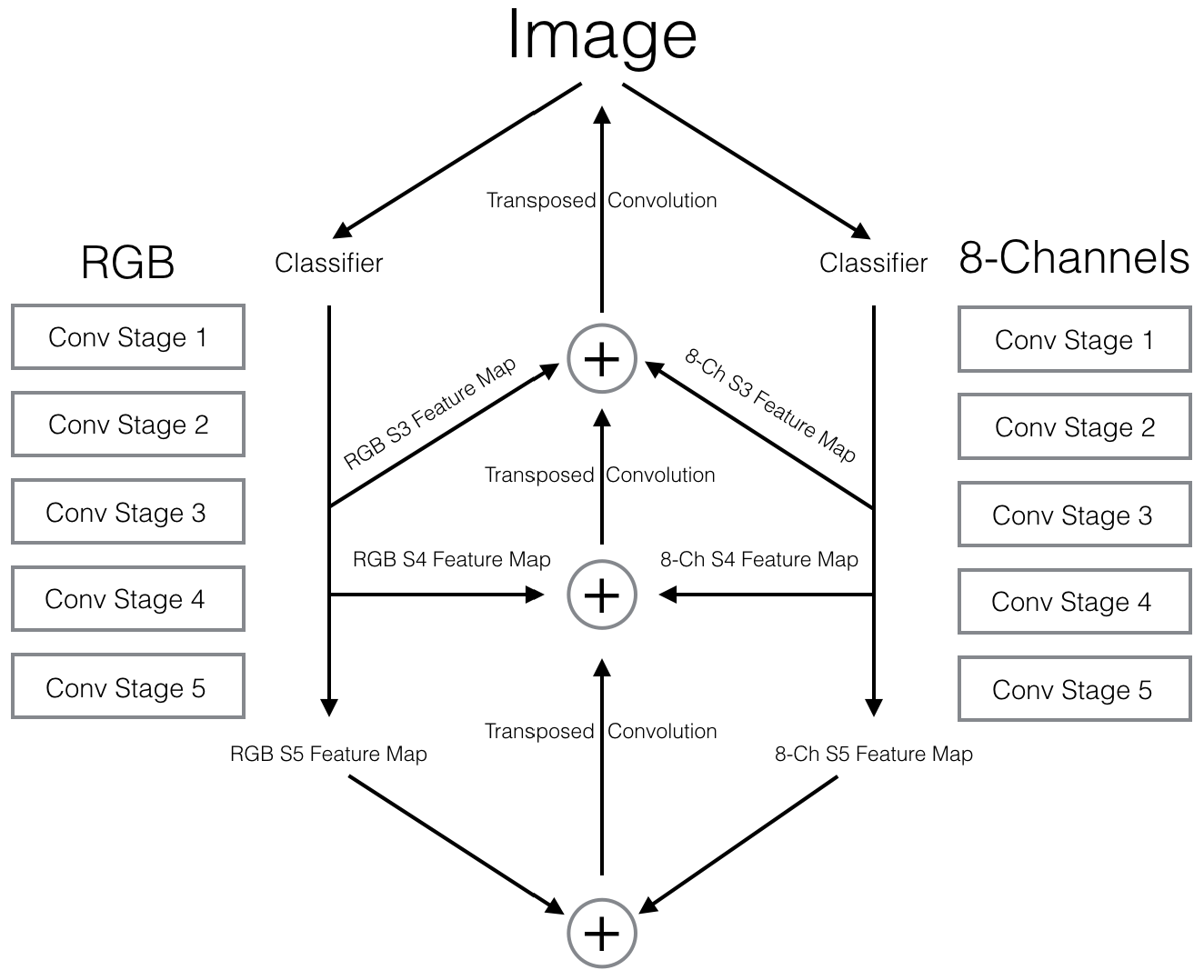
Let’s break that bad boy down by first looking only at the RGB side. For this, I used a vanilla ResNet classification backbone with the final average pooling and dense layers chopped off. The five stages in the diagram represent different spatial resolutions as the network progresses from the original input size to the final coarse resolution. Within each stage there are several convolutional layers (as well as batch normalization, RELU activations, and residual connections) that have been abstracted away from the diagram. The interested reader can learn more about ResNet here.

Since we need a classification score for each individual pixel–as opposed to a single score for the entire image–we must somehow upsample the coarse representation from stage 5 back to the original size. The goal is to do this while keeping as much of our learned information as possible. To accomplish this, we first 2x upsample the stage 5 output via an operation known as a transposed convolution (bilinear upsampling is also fairly common). We run a 1x1 convolution on the result of this operation as well as on our feature map from stage 4. Since these tensors are of the same resolution, we add the results and 2x upsample again, performing the same operations at the stage 3 level. We could keep going, but the FCN paper stops at this point, citing diminishing returns. From here, we simply upsample back to the size of the original image.

We’re almost done!

We can follow the exact same procedure to include the 8-channel network, only instead of our single combination of the feature maps from the various convolutional stages with the appropriate upsampled resolution, we add together the corresponding feature maps from both networks along with the upsampled scores. As a final addition, we combine the stage 5 scoring outputs from each network before the initial transposed convolution.

And there you have MetisNet!

Made at .

Note the resemblance… :astonished:

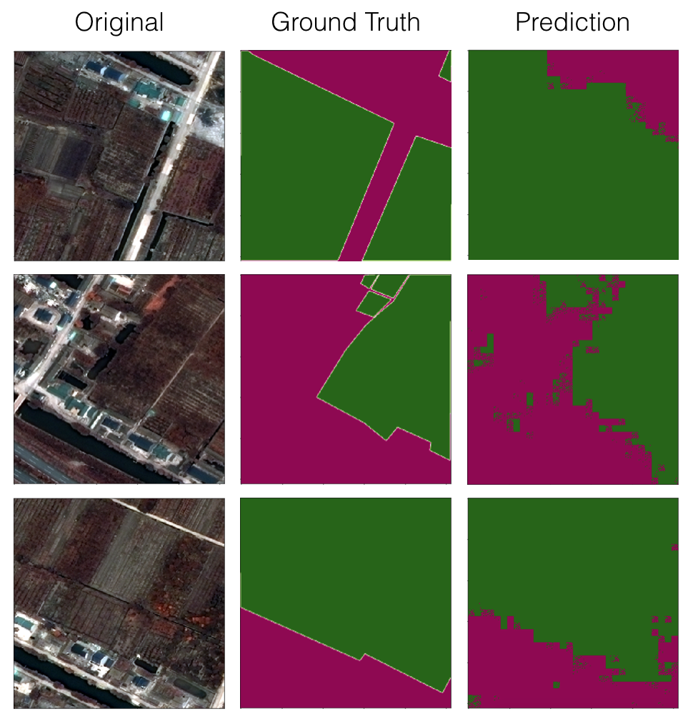
Some Results

I leave you with a few cherry-picked results to show just how awesome MetisNet performed. (In all seriousness, I was actually happy with the results but these three examples were definitely the most interesting.)

For full code from this project as well as additional commentary, please see this GitHub repo.